Predicting Fair Market Value in NCAA Basketball Head Coaching Salaries

By: Drs. Ryan Brewer, Chad McEvoy, Nels Popp, and Galen Clavio.

Background

Proper valuation of a coach by athletic directors (ADs) can help to decide what compensation level is reasonable and fair, in accord with market data, and in concert with the likely predicted performance of a given coach. The goal of this study is to provide athletic directors and other stakeholders of college basketball programs with a tool to improve their capacity for determining an appropriate level of annual compensation for a head coach having at least three years of head coaching experience. ¹

This study extends beyond traditional nonprofit executive compensation studies – which are fundamentally limited to providing market-comparative data across certain qualitative descriptors. Rather than merely report means, medians, highs, and lows, we also have investigated certain performance parameters that would predict market compensation levels. These predictors provide ADs with some insights when setting compensation levels for a particular college coach. ²

In this study, we utilize executive compensation practices and apply multiple regression analysis to develop a men’s college basketball Head Coaching compensation valuation formula. The study serves two purposes. First, the model empirically examines which factors are most relevant in determining the financial value of head men’s basketball coaching contracts. Second, the resulting model allows for the prediction of the compensation for these coaches based on coaches’ individual backgrounds.

Results

Considering all 193 coaches and their respective performance and revenues numbers, the following formula would establish a basis for the annual compensation level of a head coach in Division I men’s basketball:

Coach’s Salary is predicted by → 

3,629 x Lifetime NCAA Success +

189,794 x Lifetime Wins-Losses Percentage +

0.074478 x Basketball Revenues at the Proposed Job

Limitations

Certainly, no single study is capable of precisely predicting the market value of something as dynamic and multivariate as a coaching personality. Clearly, the values of all entities operating within service and product markets change through time, which can affect the reliability of a given valuation model. As is always the case in conducting any valuation analysis, the authors caution that methods and inputs can change over time, which could materially limit the ability of any predictor model to assess value, whether for a capital asset, a security, or for the compensation platform of a head basketball coach.

Using data in two of the Win AD databases (Coaches and Financials) from Winthrop Intelligence, LLC, and, secondarily, via the U.S. Department of Education’s Equity in Athletics Data Analysis (EADA) reports, we examined 193 current NCAA Division I men’s basketball head coaches. We also used historical coaching performance data for all coaches in the study (again, sourced from the Win AD Coaches database), such as a lifetime NCAA performance score, lifetime win-loss records, lifetime RPI, and lifetime APR. Ultimately eight variables were entered into the model.

Variables

The model included seven (7) predictor variables and one (1) dependent variable. The summary statistics are included for the entire sample for each predictor variable. These statistics include the average, high, low, and standard deviation. ³ Each variable is discussed in turn.

NCAA (used in the predictive model) –

Lifetime NCAA Tournament success factor. For every head coach, for all of the years where data was provided (Winthrop, 2013), it was noted if the team under the direction of the corresponding coach made it into the NCAA Division I Men’s Basketball Tournament (“March Madness”). The numbers here lag one year behind program revenues and compensation numbers, as strictly the prior performance should predict the consequent pay. Points were assigned to each coach as follows: Five (5) points for getting a bid and playing a round-of-64 game; Ten (10) points for winning game 1 and appearing in the round-of-32 game; Twenty (20) points for making it into the Sweet Sixteen; Twenty-five (25) points for making it into the Elite Eight; Fifty (50) points for making it to the Final Four; and One Hundred (100) points for winning a championship. All points were deemed to have indefinite shelf life without discounting the time value of winning. The average number among all 193 head coaches was 47, with a high of 800, and a low of 0. The standard deviation was about 96.

WLO (used in the predictive model) –

The “win-loss-overall” variable included all wins and all losses recorded as a head coach. The numbers here lag one year behind program revenues and compensation numbers, as strictly the prior performance should predict the consequent pay. The mean was 0.56, the high was 0.82 and the low was 0.18. The standard deviation was 0.11.

WLC –

The “win-loss-conference” variable included all wins and losses in conference play, for all teams coached as a head coach, with all conference wins coalesced. The numbers here lag one year behind program revenues and compensation numbers, as strictly the prior performance should predict the consequent pay. The mean was 0.55, the high was 0.91, and the low was 0.15. The standard deviation was 0.14.

APR –

The “academic progress rate” was the average lifetime number for each head coach overall, lagging one year behind program revenues and compensation numbers. This reflects the team’s average college credit accrual per player, and their collective graduation rate. The mean was 932, the high was 999 and the low was 863. The standard deviation was 28.41.

RPI –

The “rating percentage index” was the average lifetime number for each head coach overall, lagging one year behind program revenues and compensation numbers. This number reflects the strength of schedule and wins and losses within that context. Developed in 1981, the index comprises a team’s winning percentage (25%), its opponents’ winning percentage (50%), and the winning percentage of those opponents’ opponents (25%). The opponents’ winning percentage and the winning percentage of those opponents’ opponents both comprise the strength of schedule (SOS). Thus, the SOS accounts for 75% of the RPI calculation, and RPI is 2/3 its opponents’ winning percentage and 1/3 its opponents’ opponents’ winning percentage. The mean was 144, the high was 340, and the low was 5. The standard deviation was 7.7.

Experience –

The total number of years in the Head Coach position, only. The number of years of head coaching experience each coach accrued was also collected. Of the 193 coaches, the minimum experience seen was three (3) years, while the most experienced head coach had accrued thirty-eight (38) years on the bench. Experience as an assistant or associate head coach was excluded from our analysis, both in terms of the “experience” variable, as well as the other variables, which are described below.

Program Revenue (used in the predictive model) –

The estimate was made by summing the pro rata percentage of non-allocated revenues with those revenues directly attributed to men’s basketball, as reported on the annual NCAA Financial Reports (Winthrop, 2013), or in limited cases from the EADA cutting tool (2013). The pro rata percentage of non-allocated revenues was established by assessing the fraction of total allocated revenues within each athletic department that comprised men’s basketball allocations, and multiplying this fraction by the non-allocated revenues. Furthermore, no adjustments were made for non-cash value attributions such as goodwill to the university, the Flutie Effect, differential state appropriations, or other indirect revenues arising from sport presence. Program revenues ranged from a low of $230,633 to a high of $54,434,684.

Current Head Coach Compensation (Response Variable) ⁴ –

The current salary includes the number taken from the NCAA Financial Reports describing “head coach total pay for (men’s basketball) in (2011-2012).” Therefore, the “current head coach compensation” is a comprehensive annual number—money actually paid to the coach as a result of his service as Head Coach (a better overall figure because of the complexity of each contract). For the entire group of N = 193, the mean total compensation was $821,746, with the high being $5,248,000, and the low being $86,464. The standard deviation was $970,699.

Together, these three variables explain 89.2% percent of the variability among coaches’ compensation. Based on the model’s results, the following were the top 12 highest predicted compensation figures for the 2011-12 season:

Top 12 Highest Predicted Compensation Figures for the 2011-12 Season

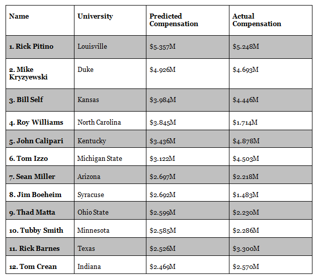
As shown from the table above, the model suggests that seven coaches are compensated at levels less than what was predicted, while five coaches are compensated above the predicted amounts. Of course, there is a range of reasonable compensation that might be described by the predicted amount, plus or minus some fraction of the predicted number.

It is important to note the size of basketball revenue for each school was an important predictor variable in the regression model. For example, Sean Miller is an outstanding basketball coach, but may not possess the level of career success shared by many of the other elite coaches on this list above. We noted that according to a recent report from the Wall Street Journal, ⁵ the Arizona’s men’s basketball program is one of the five most financially valuable college basketball programs in the U.S., providing support for our model’s relatively high predicted compensation level for Miller. In essence, programs having strong revenues and cash flow more commonly support higher head coaching salaries, while the on-court performance of winning percentage and making deep runs into the NCAA tournament are also keys to explaining higher salaries.

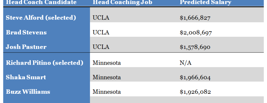
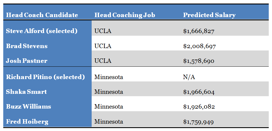
Beyond measuring a snapshot in time about a compensation level being above or below the predicted value, the model has the ability to suggest an appropriate salary range for current head coaches who are hired at another institution, based on current market trends and standards. ⁶ For example, let’s take a look at two vacancies filled this spring at UCLA and the University of Minnesota.

At UCLA, some of the candidates initially included Steve Alford (New Mexico), Brad Stevens (Butler), and Josh Pastner (Memphis). Alford was hired for the position, while Shaka Smart (Virginia Commonwealth), Buzz Williams (Marquette), and Fred Hoiberg (Iowa State) were initially to be candidates at Minnesota. Ultimately, Richard Pitino, the head coach at Florida International University last year, was hired to lead the Golden Gophers’ program.

We have used our model to predict fair market values of compensation for the Candidates for the Head Coach position at UCLA and Minnesota, as shown below.

Predicted Compensation for Head Coaching Candidates at UCLA and Minnesota

We recognize there are many factors operating in the real world beyond any model, no matter how well intentioned and empirically sound. With this paper and the model we present, it is our aim to provide additional information that can help athletic directors make investments and the most informed hiring decisions. We also acknowledge that in some hiring scenarios, market forces and trend data play lesser roles compared to the intangibles of timing, personality, and program fit. In some cases, comparative data takes a back seat to ensuring the hiring of a coach deemed to be the best overall match, or protecting against a valued coach’s departure. However, knowing the fair market compensation level for a given coach—within the context of that head coaching position—helps shape the intangibles of hiring and compensation.

RYAN BREWER

ASSISTANT PROFESSOR OF FINANCE

INDIANA UNIVERSITY-PURDUE UNIVERSITY COLUMBUS

 

 

CHAD MCEVOY

PROFESSOR

SYRACUSE UNIVERSITY

 

 

NELS POPP

ASSISTANT PROFESSOR OF SPORT MANAGEMENT

ILLINOIS STATE UNIVERSITY

 

 

GALEN CLAVIO

ASSISTANT PROFESSOR OF KINESIOLOGY

INDIANA UNIVERSITY BLOOMINGTON